 The Met Office NERC Cloud model (MONC) is an atmospheric model that we developed with the Met Office between 2014 and 2016, and I was the main developer of in this period. Since then we have undertook some general maintenance activities on the code-base and also used it as a technology demonstrator. This is now one of the main high-resolution atmospheric models used by the Met Office and UK scientists, and is controlled by a steering group comprising the Met Office, Universities of Leeds and Reading, and NCAS. The code is BSD licenced, and hosted here. An account is required for access to the Met Office science repository, and it is this version we strongly recommend people use, but there is a also a previous version here.
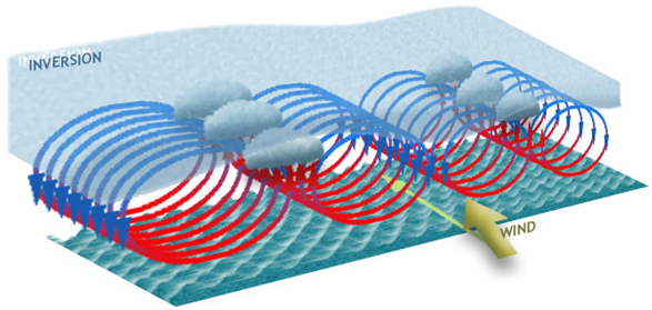 The model provides a Large Eddy Simulation (LES) approach to atmospheric modelling, where Navier–Stokes equations are solved to resolve the most important turbulent features at a specified resolution, with other facets parameterised. This code replaced a previous mode, the Large Eddy Model (LEM) from the 1990s, with the aim of developing an approach that could fully exploit modern supercomputers and leverage modern software engineering techniques. A stencil based code, with 2D domain decomposition, the model enables a step change in scientific capability. For instance the previous model was capable of modelling systems comprising around ten million grid points, whereas MONC routinely handles billions of grid points. This enables larger domains, at higher resolution to be modelled, but also much quicker where runs usingthe LEM that would take many hours or days to complete, now take a couple of hours or less in MONC.
A toolkit for atmospheric science
Written in Fortran 2003, these model have lifetimes of up to thirty years, and an important question was how to enable generations of atmospheric scientists to develop code whilst maintaining overall quality. When one considers that people often want to use the model to explore different phenomena, which requires additional code or coupling with other models, then the ability for different aspects to be isolated from each other is really important. The approach we adopted is illustrated below, where the vast majority of the model is provided as independent, pluggable components, and this diagram illustrates a subset of the components shipped with the model. These are all independent from each other, and using Fortran procedure pointers implement up to three optional callbacks. These callbacks are subroutines that are optionally called on model initialisation, for each timestep, and on model finalisation, with the current state of the simulation provided as a Fortran derived type. Conceptually, the user can select which of these are active, for instance different scientific components for different runs, and furthermore if they wish to replace certain aspects (e.g. a GPU or FPGA implementation of specific functionality), then one just needs to develop their own component, enable it, and disable the existing one.
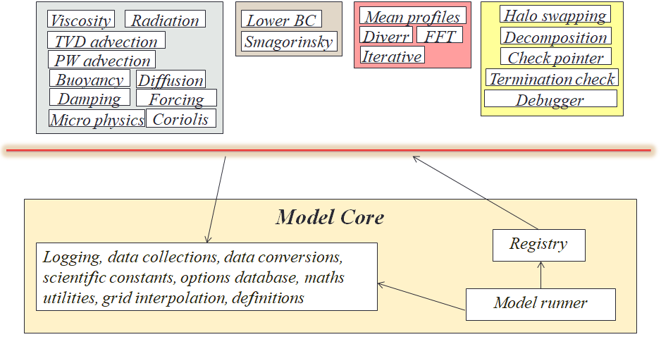
Below the red line in the image above is the model core, which is a small amount of bootstrapping, utility, and component control functionality. Whilst new components can be freely added, the model core is more protected, with the idea being that it provides the underlying mechanism which enables the execution of components and hence all the science that they provide.
A challenge for data analytics
 The scientists are not so interested in the prognostic values that are directly generated from the code, but instead higher level information derived from this known as diagnostics. Previous generation models, such as the LEM, would perform a data analytics step inline with computation, typically after calculates have completed for each timestep. This can be very communication heavy, and even with much smaller data sizes, was a source of significant overhead for these older models. Therefore we adopted an in-situ approach, where cores of a processor are shared between computation and data analytics, typically with one data analytics core servicing the other computational cores per NUMA region. These computational cores fire and forget the raw prognostic data to their analytics core, with this then performing analysis and necessary calculations, before writing to file. Whilst there are some frameworks that provide in-situ data handling, such as XIOS, typically these are much more focused around IO, rather than the analysis itself, and furthermore we found that there was no existing technology that could support dynamic timestepping, checkpoint-restart of the data analytics, bit reproducibility, and scaling.
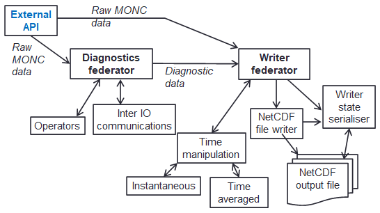 We therefore developed a bespoke in-situ data analytics approach, which is organised as a data analytics pipeline illustrated to the left. There are two main federators here, one for generating the diagnostics (the data analytics), and one for performing IO (file writing), each containing sub-functionality. Not only is this how the code is structured, but also the abstraction provided to the user when they write data analytics configurations (in XML) to describe how to transform their raw prognostic data into higher level diagnostics. There were a few major challenges here, the first one was that of time manipulation where each individual value isn’t necessarily desired but instead averages over time (e.g. the average over every five minutes.) Because timestepping is dynamic (the amount of time each timestep represents changes based upon numerical stability), it is not possible to know ahead of time exactly how many contributions there will be to each value, and edge cases such as when there are no contributions or values cross IO write boundaries. Another major challenge is that of checkpoint-restart, where due to the typical 24 hour limit on HPC jobs, the code will write out its entire state, for instance after 23 hours of run, and then automatically reschedule itself to restart based on this state for another day of execution. However, the in-situ data analytics approach is highly asynchronous, where for performance reasons we promote the loose coupling of analytics cores and numerous communications active at any one point in time. But to perform this checkpoint-restart, then at a specific point in time the state must be entirely known. To address this, for checkpointing the code waits at a specific point in time until all required values at that point are available to the write federator, which is then locked and serialised for writing.
Event based communications
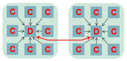
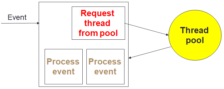 To provide maximum performance, it is important that the in-situ data analytics does not stall the computational cores. The computation itself can be at slightly different stages from core to core, and as such analytics cores need to be able to handle the processing and communication of many different pieces of independent data concurrently. We realised that the optimal approach was that of Event Based Coordination (EBC), where much of the processing is driven by the arrival of events. This is illustrated to the right where a core, for instance the root of a reduction, receives an event which is then allocated to an idle thread which processes the event. This also helps us with bit reproducibility, where for some event handlers we must enforce event ordering (e.g. the processing of data in a strict timestep order), and where this matters we queue up events that arrive out of order for processing later. Within the Fortran code of the federators, this is organised as callbacks, where communications provide an additional unique identifier and handling subroutine. An example of this is illustrated below, where there is a reduction of some data, summing up the result with the root being rank zero. The unique identifier is a concatenation of the field name and timestep, with the handling subroutine then executed on the root when the reduction has completed. This handler is stateless, with the data and some context provided to it.

The proof is in the pudding
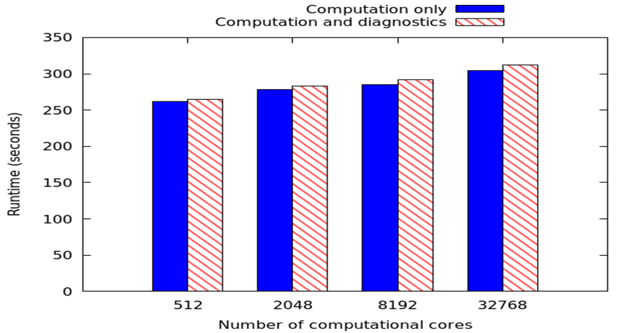 The graph to the left represents weak scaling on a Cray XC30 using a standard MONC stratus cloud test case and 65536 local grid points per process. There are 232 diagnostic values which require calculation every timestep, with time averaged over 10 model seconds. A result file is written every 100 model seconds, and the run terminated after 2000 model seconds. We are increasing the number of computational cores and comparing performance between no analytics (or IO) in blue, and analytics with IO enabled. It can be seen that when using our approach the overhead of enabling analytics is minimal, around 8 seconds with 32768 computational cores. It should be noted that in this experiment the number of computational cores is fixed, and we have a ratio of 11 computational cores to 1 analytics core. Therefore with 32768 computational cores, when we enable data analytics there are around 3500 extra analytics cores, and thus in total the model is running over around 36000 CPU cores.
A test-bed to explore other technologies
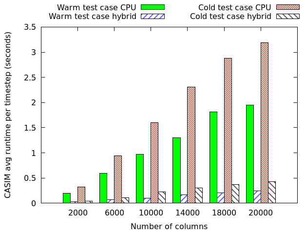 We have also used MONC as a test-bed to explore the role of other technologies, namely GPUs and FPGAs, in accelerating these sorts of workloads. The GPU work was conducted in 2015 and 2016 as part of two MSc dissertation projects, where my students accelerated the advection component of MONC and the CASIM microphysics submodel. This was all done using OpenACC on Piz Daint, a Cray XC50, and is an example of where our toolkit approach worked well, as the student was able to simple disable the existing component and replace it with their accelerated version. A comparison between two CASIM test-cases (warm, which is water above freezing only, and cold which includes all water states) on a P100 GPU and Haswell CPU is illustrated to the right. This is reporting the time per timestep, where lower is better and it can be seen that the GPU provides performance benefits, albeit with some caveats that we explore in the associated paper.
We also used MONC to explore the use of reconfigurable architectures, specifically FPGAs, in accelerating advection. This was done on the Xilinx Kintex UltraScale of an AlphaData ADM8K5, and we found here that the devil is in the detail. There was around a 500 times difference in performance between the first version of our (High Level Synthesis) HLS kernel, and the final optimised version that we ended up with. The entire code structure had to be rethought and rewritten in dataflow style, as illustrated by the diagram below where each box is a dataflow region that contains a pipeline operating on slices of the domain. It was worth it however, where we achieved between 1.22 and 2.59 times the performance of an 18-core Broadwell CPU at less than half the energy usage.

Related publications
- It’s all about data movement: Optimising FPGA data access to boost performance. Brown, N. & Dolman, D. In IEEE/ACM International Workshop on Heterogeneous High-performance Reconfigurable Computing (H2RC) (more info)
- Exploring the acceleration of the Met Office NERC Cloud model using FPGAs. Brown, N. In LNCS High Performance Computing: ISC High Performance 2019 (more info)
- Massively parallel parcel-based simulation of moist convection. Boeing, S., Gibb, G., Brown, N., Weiland, M. & Dritschel, D. G. In EGU General Assembly 2019 (more info)
- Leveraging MPI RMA to optimise halo-swapping communications in MONC on Cray machines. Brown, N., Bareford, M. & Weiland, M. In Concurrency and Computation: Practice and Experience (more info)
- In situ data analytics for highly scalable cloud modelling on Cray machines. Brown, N., Weiland, M., Hill, A. & Shipway, B. In Concurrency and Computation: Practice and Experience (more info)
- Porting the microphysics model CASIM to GPU and KNL Cray machines. Brown, N., Nigay, A., Weiland, M., Hill, A. & Shipway, B. In proceedings of the Cray User Group (CUG) (more info)
- MONC – highly scalable cloud modelling on the latest supercomputers. Brown, N. In Computing Insight UK (more info)
- A highly scalable Met Office NERC Cloud model. Brown, N., Weiland, M., Hill, A., Shipway, B., Maynard, C., Allen, T. & Rezny, M. In proceedings of the 3rd International Conference on Exascale Applications and Software (more info)
- A directive based hybrid met office NERC cloud model. Brown, N., Lepper, A., Weiland, M., Hill, A., Shipway, B. & Maynard, C. In proceedings of the Second Workshop on Accelerator Programming using Directives (more info)